A Little Bit of Galois Theory

This chapter is no  introduction into Galois theory, let alone an easy to grasp introduction for high-school students. As a matter of fact, I do not feel competent for such a task. It isn't by chance, that Galois theory is said to be a rather technical discipline within mathematics. In Germany students will hear about it at the earliest in their second year at university as part of a lecture in abstract algebra. The technical character of the matter shows up in the fact, that many of the theorems start with a long list of preconditions, which must be checked one by one, if the theorem shall be applied in a special case. And it's not sure that you succeed with these checks without trouble (see the quotation of Ian Stewart below).

As has been said in the preface, the intention of this chapter is, to demonstrate the connections between Galois theory and Gauss' classical approach to cyclotomy for those, who already know a little bit of Galois theory. Hence, we will feel free to state results without proving them or to use terms without defining them throughout this chapter.

If you want to recapitulate proofs or to brush up your knowledge generally, you may consult the literature. Besides the classical textbooks there are a lot of lecture notes in the web, which can be downloaded for free, and which are of no lesser quality than that of printed media. A search with the keywords galois theory, introduction, lecture note  will uncover many a gem. If you prefer paper, you may have a look into the book [Stewart 1988] about Galois theory, which differs from the very technical approaches by its relaxed style. The book of [Bewersdorff 2006] addresses explicitely the reader without previous knowledge and presents the construction of regular polygons in unusual detail.

Nevertheless, the reader without background knowledge is also encouraged to skim through this chapter. After all, you may inform yourself about the principles of operation of an mp3-player, without understanding all the details of the compression algorithm or being an expert of the quantum physics of flash memory.

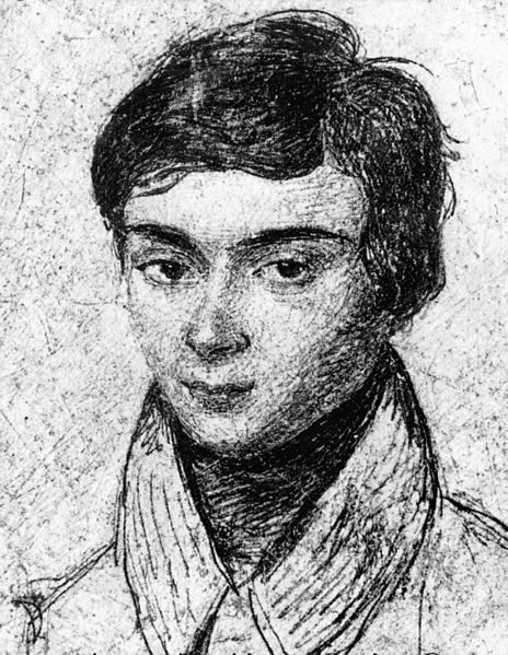
The Galois theory dates back to Evariste Galois (1811-1832), whose fierce and violently terminated short life made him a kind of rock star among the mathematicians. Galois discovered that the question, whether the zeroes of a polynomial can be represented by radical expressions  or roots, can be answered by looking at the symmetries of these zeroes. In modern terminology ths symmetry is given by a certain group, the Galois group of the polynomial, and the polynomials themselves are hidden behind certain fields, namely their splitting fields.

Solvability of Polynomials by Radicals

Let's start right away with the theorem, that in a systematic approach is presented near the end of a series of lectures, with the main theorem about the solvability of polynomials by radicals:

In our special case the polynomial $f$ is of course \[X^n - 1 \eqndot\] Its coefficients are in the field $\mathbb{Q}$ of rational numbers, which luckily has characteristic zero (that is $\sum^n1 \neq 0$ for all $n \in \mathbb{N},$ if $0$ and $1$ are the identity elements of addition and multiplication respectively in this field). Furthermore, we are not interested in any  solution of this polynomial by radicals, but in a solution by nested square roots.

The Galois group is defined in the first place only for field extensions $L:K$ and not for polynomials with coefficients in $K$. It's the group of automorphisms  of the field $L,$ which keep the elements of $K$ fixed. Remember: automorphisms of fields are bijective maps $\tau$ of a field onto itself, that respect the addition and multiplication in this field, in other words with $\tau(a+b) = \tau(a)+\tau(b)$ and $\tau(ab) = \tau(a)\tau(b)$ for all $a,b$ in the field. The definition of solvability of a group doesn't bother us in the moment, we will explain that later.

The Galois group of a polynomial with coefficients in $K$ is now defined simply as the Galois group of the splitting field  of this polynomial, that is the smallest extension field of $K,$ in which the polynomial splits into linear factors. The splitting of our polynomial into linear factors has already been presented in chap.3: \[X^n - 1 = (X-1)(X-\zeta)(X-\zeta^2)\cdot \dots \cdot(X-\zeta^{n-2})(X-\zeta^{n-1})\eqncomma\] with $\zeta^k$ being $n$th roots of unity.

Adding all this roots of unity to $\mathbb{Q},$ the technical term is to adjoin  them, yields a field, in which the polynomial $X^n -1$ surely splits. But that would be using a sledge-hammer to crack a nut, because all these roots of unity are powers of a single $\zeta.$ These powers are created automatically in the process of adjunction, because the extension field allows unlimited multiplication. Therefore, it suffices to adjoin the root of unity $\zeta,$ and one writes $\mathbb{Q}(\zeta)$ for this extension field.

Degree of the Field Extension $\mathbb{Q}(\zeta)$

For what follows the degree  of the field extension by a splitting field (esp. $\mathbb{Q}(\zeta)$) over the base field (esp. $\mathbb{Q}$) is of utmost importance. The degree of a field extension $L:K$ is the dimension of $L$ over $K,$ when $L$ is considered as $K$-vector space.

At this moment a reader, who never has heard anything about Galois theory, will share our opinion, that it is a rather technical theory. Perhaps, it may help to remark, that one simply forgets the multiplication defined in $L,$ when looking at it as a $K$-vector space, and searches an as small as possible set of elements in $L$ (the basis), such that every element in $L$ can be represented as linear combination of elements of this set with coefficients in $K$. The number of elements of the basis is the dimension of the vector space.

An important theorem of Galois theory is, that the degree of a field extension, which is generated by adjunction of an algebraic element $\rho$ to the base field $K$ equals the degree of the minimal polynomial  of $\rho$ in $K[X].$ In this regard an element is called algebraic, if it's a zero of any  polynomial in $K[X].$ Hence, our $\zeta$ as zero of $X^n-1$ in $\mathbb{Q}[X]$ is definetely algebraic.

However, the mimnimal polynomial of $\zeta,$ that is the normalized polynomial of minimal degree, having $\zeta$ as one of its zeroes, is not at all $X^n-1.$ By the factorization \[X^n - 1 = (X-1)(X-\zeta)(X-\zeta^2)\cdot \dots \cdot(X-\zeta^{n-2})(X-\zeta^{n-1})\] it follows, that $\zeta$ is also a zero of \[(X-\zeta)(X-\zeta^2)\cdot \dots \cdot(X-\zeta^{n-2})(X-\zeta^{n-1})\eqndot\] This polynomial, that we have called cyclotomic polynomial in chap.3 has degree $n-1.$

If $n$ is prime, we are done, because in this case the above polynomial is irreducible  and thus really the cyclotomic polynomial. In chap.3 we already have remarked in a footnote, that in case of $n$ being composite only a certain factor of the above polynomial is called cyclotomic polynomial. To be precise, it's the largest irreducible factor. The reason for this will become clear soon.

If $n$ is composite, the powers of a root of unity $\zeta^d$ with $d|n$ generate only a part of the complete set of all roots of unity, because by $n = d\cdot k$ we have \[(\zeta^d)^k = \zeta^n = 1\] with $k \lt n.$ These $\zeta^d$ don't contribute to the generation of the splitting field. More interesting are the powers of $\zeta$ with exponents relative prime to $n,$ the so called primitive  roots of unity, because these are of order $n,$ in other words, their powers generate all  roots of unity.

Hence, searching for the minimal polynomial of $\zeta,$ it seems to be a good idea, to concentrate on a polynomial, whose zeroes are just these primitive roots of unity, because these roots suffice to generate the splitting field. Because their number is smaller as $n,$ one may hope, that this polynomial is of smaller degree than $n-1.$ The most simple way to get such a polynomial is to take the product of the particular linear factors: \[\Phi_n = \prod_{(q,n)=1,q\leq n}(X-\zeta^q) \eqncomma\] with $(q,n)=1$ as abbreviation of $\gcd(q,n) = 1,$ hence the product runs over all $q\leq n,$ relative prime to $n.$ All one has to do is only  to prove, that the polynomial $\Phi_n$ has coefficients in $\mathbb{Q}$ after expanding the linear factors.

You won't be surprised to hear that this really can be done, moreover the coefficients actually are in $\mathbb{Z}.$ The proof is not too complicated and can be found in the literature, given above. There you will also find the proof, that $\Phi_n$ is irreducible and thus the minimal polynomial of $\zeta.$ $\Phi_n$ is called the $n$th cyclotomic polynomial  and is equal to \[(X-\zeta)(X-\zeta^2)\cdot \dots \cdot(X-\zeta^{n-2})(X-\zeta^{n-1})\] if $n$ is prime.

Wantzel's Theorem

Now we know that for all $n$, prime or composite, the degree of the field extension $\mathbb{Q}(\zeta)$ equals the degree of the polynomial $\Phi_n,$ if $\zeta = \zeta_n$ is a $n$th root of unity.

By construction of $\Phi_n$ its degree is the number of different positive integers $q \leq n,$ with $q$ relative prime to $n.$ To compute this number, already Euler introduced an arithmetic function, the Euler totient function  $\varphi(n)$: \[\varphi(n) := \#\{q \leq n: (q,n)=1, q,n \in \mathbb{N}\}\eqndot\] If $n=p$ is a prime we have $\varphi(p) = p-1,$ because all positive integers $1,2,\dots,p-1$ are relative prime to $p.$

Also for powers of a prime, the Euler totient function can easily be computed, it's \[\varphi(p^k) = p^{k-1}(p-1)\eqncomma\] because a number $q \leq p^k$ is relative prime to $p^k,$ if and only if it is no multiple of $p.$ Of these multiples there are $p^{k-1},$ precisely \[1p,\quad 2p,\quad 3p,\quad \dots,\quad p^{k-1}\cdot p = p^k \eqncomma\] being less or equal $p^k.$ So there remain \[p^k-p^{k-1} = p^{k-1}(p-1)\] positive integers less or equal $p^k,$ which are relative prime to $p^k.$

A little bit more complicated is the proof that the Euler totient function is multiplicative, in other words that for relative prime $a,b \in \mathbb{N}$ we have \[\varphi(a\cdot b) = \varphi(a)\cdot\varphi(b)\eqndot\] You will find a proof in the aforesaid literature.

From the multiplicativity it follows immediately the value of $\varphi(n)$ for all $n \in \mathbb{N}.$ Because every $n$ has a unique decomposition into prime factors \[n = p_1^{k_1}\cdot p_2^{k_2} \cdot \dots \cdot p_s^{k_s} \eqncomma\] one has \[\varphi(n) = p_1^{k_1-1}(p_1-1) \cdot p_2^{k_2-1}(p_2-1) \cdot \dots \cdot p_s^{k_s-1}(p_s-1)\eqndot\]

In summary we have the following intermediate result:

It turns out that only by inspecting the degree of a field extension, without going into details about the Galois group and their solvability, an important result can be achieved. To do so, we go back to our square root expressions. We want to solve the polynomial $X^n -1$ by nested square roots. Every square root is a zero of a quadratic minimal polynomial, so it must belong to a field extension of degree 2. Hence, the splitting field of $X^n-1$ is the last field within a chain of field extensions, each of degree 2. By another, relatively simple proposition of Galois theory one has on the one hand \[\mathbb{Q}(\zeta) : \mathbb{Q} = \varphi(n)\] and on the other hand \[\mathbb{Q}(\zeta) : \mathbb{Q} = 2^r \] with a suitable $r \in \mathbb{N}.$ Equating both expressions yields: \begin{align*} 2^r &= p_1^{k_1-1}(p_1-1) \cdot p_2^{k_2-1}(p_2-1) \cdot \dots \cdot p_s^{k_s-1}(p_s-1)\eqncomma \\ 2^r &= 2^{k_1-1} \cdot p_2^{k_2-1}(p_2-1) \cdot \dots \cdot p_s^{k_s-1}(p_s-1)\eqncomma \end{align*} if we separate the even prime $2.$

This equation can only be solved, if for every odd prime factor we have $p_i^{k_i-1} = 1,$ because a power of two can have no odd prime factors, and if $p_i-1$ is itself a power of two, thus $p_i$ being a Fermat prime. The exponent of $2,$ however, may be any positive integer or zero.

The $p_i$ come from the prime factorization of the number $n$ of vertices of the regular polygon. So we have shown that a regular $n$-gon can be constructed with ruler and compass, only  if the prime factorization of $n$ is \[n = 2^k \cdot p_1 \cdot p_2 \cdot \dots \cdot p_s\] with different Fermat primes $p_i.$

That is nothing else as the reverse of Gauss' cyclotomic theorem, and it has been proved, as we have already mentioned in the preface, by Wantzel in 1837 (of course in a classical manner without Galois theory). Obviously, Gauss knew this theorem and even had a proof, a fact that can be deduced from several remarks in [Gauß 1801], but he never published it. A proof of Wantzel's theorem without using Galois theory can be found in [Hudson 1969].

In particular, all regular polygons with the number of vertices equal to $p^k,$ $p$ an odd prime and $k>1$ are not  constructible. Thus, our restriction to pure prime numbers in chap.4 is justified retrospectively.

Solvability of Groups

The other and original implication of the Gauss' theorem, that every regular polygon with $n = 2^k \cdot p_1 \cdot p_2 \cdot \dots \cdot p_s$ can in fact be constructed with ruler and compass, cannot be integrated into Galois theory without considerations about the solvability of groups. Here we may restrict ourselves to polygons with a prime number of vertices, because we have already shown that the constructibility of the $n$-gon follows from the constructibility of each of the $p_i$-gons.

In the framework of Galois theory we have to show, that the cyclotomic polynomial $\Phi_p,$ with $p$ a fermat prime, is solvable by quadratic radicals. By the main theorem about solvability of polynomials this is equivalent to showing the solvability of the Galois group of the splitting field of $\Phi_p.$

A group $G$ is said to be solvable, if there is a chain of subgroups \[I = G_0 \subseteq G_1 \subseteq \dots \subseteq G_s = G\] with $G_i \lhd G_{i+1}$ for $i = 0,1, \dots , s-1$ and all quotient groups $G_{i+1}/G_i$ being Abelian. The symbol $G_i \lhd G_{i+1}$ indicates that $G_i$ is not only a subgroup but a normal  subgroup in $G_{i+1}.$

This, once again, is one of those deterrently technical definitions. However, it is not necessary to understand every detail of it, because it can be proved, that generally all groups with $p^k$ elements (one speaks of groups of order $p^k$), with $p$ being a prime, are solvable. Moreover, it turns out that the normal subgroups $G_i$ in the chain are of order $p^i.$

And now we deploy the heaviest artillery of Galois theory, namely its main theorem (not to be confused with the main theorem about the solvability of polynomials):

Again, it will not be a surprise, that one can prove the necessary conditions of finiteness, separability and normality for the field extension $\Phi_p : \mathbb{Q}$ (as a convenient abuse of notation we have denoted the splitting field of $\Phi_p$ also by $\Phi_p$). The field extension has degree $2^k$ by requirement, thus the Galois group of this extension is of order $2^k,$ and thus is solvable as a group of prime power order.

Consequently, there exists a chain of normal subgroups $G_i$ within the Galois group, and each of these is of order $2^i.$ By the main theorem there exists a corresponding chain of intermediate fields \[\mathbb{Q} = G_s^\dagger \subseteq G_{s-1}^\dagger \subseteq \dots \subseteq G_1^\dagger \subseteq G_0^\dagger = \Phi_p\] and the degree of the field extension $\Phi_p : G_i^\dagger$ is $2^i.$ It follows that the degree of the field extension $G_i^\dagger : G_{i+1}^\dagger$ must be $2.$ Hence, $G_{i}^\dagger$ is a splitting field of a polynomial of degree $2$ with coefficients in $G_{i+1}^\dagger.$ But that's exactly, what we wanted to show.

Where Are the Gaussian Periods Gone?

So far, our considerations demonstrate the whole power of Galois theory, but also its difficulties. We arrived at the results of Gauss and Wentzel without any hint, how to find the minimal polynomials of the extensions $G_{i}^\dagger : G_{i+1}^\dagger$ in practice, or how the adjoint roots look like. This is not at all untypical in Galois theory, look at the following statement of Ian Stewart in [Stewart 1988]:

[…] it is necessary to compute the corresponding Galois group. This is far from being a simple or straightforward task, and until now we have strenuously avoided it.

Luckily, the polynomial $X^p -1$ is particularly simple. In fact, it's the most simple non trivial polynomial of degree $p$ at all. Hence, the Galois group of the field extension corresponding to this polynomial can be expected to show a comparably simple structure.

Remember that the Galois group of $\mathbb{Q}(\zeta) : \mathbb{Q},$ which we will denote by $\Gamma$ from now on, is the group of all automorphisms $\tau$ of $\mathbb{Q}(\zeta),$ keeping fixed the elements of $\mathbb{Q},$ in other words the rational numbers. Because every automorphism of $\mathbb{Q}(\zeta)$ respects the multiplication, $\tau$ is uniquely determined by its action on one  root of unity $\zeta.$

Moreover, the image of $\zeta$ under $\tau$ cannot be an element $a$ in $\mathbb{Q},$ because as an automorphism $\tau$ is an injective map, and we already have $\tau(a) = a.$ Hence, there is no other posiibility for $\tau,$ as to map $\zeta$ on another $p$th root of unity – we already have seen that by adjunction of $\zeta$ these roots are automatically generated in $\mathbb{Q}(\zeta).$ Because every root of unity is a power of $\zeta,$ it holds \[\tau(\zeta) =\zeta^\omega\] with an $\omega \in \mathbb{N},$ and by this the automorphism is completely determined.

The group operation within a group of automorphisms is nothing else as the composition of the automorphisms. So let's operate $\tau$ repeatedly on $\zeta$: $$ \begin{align*} \tau(\zeta) &= \zeta^\omega \\ \tau^2(\zeta) = \tau(\tau(\zeta)) &= (\zeta^\omega)^\omega = \zeta^{\omega^2} \\ \tau^3(\zeta) = \tau(\tau^2(\zeta)) &= (\zeta^{\omega^2})^\omega = \zeta^{\omega^3} \\ & \text{etc.} \\ \end{align*} $$ Here they are again, the summands of the Gaussian periods. Admittedly we promoted their appearance by the suggestive choice of $\omega$ for the exponent.

In chap.5 we have denoted a primitive element in $\mathbb{Z}/p\mathbb{Z}$ by $\omega.$ Taking the exponent $\omega$ in the above definition of $\tau$ as primitive element, $\tau$ will generate the whole group $\Gamma,$ because every exponent of $\zeta$ can be written as $\omega^k$ with a suitable $k$ and every automorphism in $\Gamma$ maps $\zeta$ on a power of $\zeta,$ thus being of the form $\tau^k.$

A group, generated by one element $\tau,$ is called cyclic  group, and one writes $\Gamma = \langle \tau \rangle,$ to indicate that the whole group is generated by $\tau.$ It's easy to see that also $\tau^2, \tau^4$ etc. generate groups, namely subgroups of $\Gamma,$ and it holds \[\Gamma = \langle \tau \rangle \supset \langle \tau^2 \rangle \supset \langle \tau^4 \rangle \supset \dots \supset \langle \tau^{p-1/2} \rangle \supset \langle \tau^{p-1} \rangle = 1\] Because cyclic groups are Abelian, all subgroups are normal subgroups automatically \[\langle \tau^{2^k} \rangle \lhd \langle \tau^{2^{k-1}} \rangle\] and the quotient groups are Abelian as well. Hence, we have found the chain of groups (the technical term is derived series ) that demonstrates the solvability of the Galois group $\Gamma.$

By the main theorem of Galois theory we know the corresponding chain of field extensions \[\mathbb{Q} = {\langle \tau \rangle}^\dagger \subset {\langle \tau^2 \rangle}^\dagger \subset {\langle \tau^4 \rangle}^\dagger \subset \dots \subset {\langle \tau^{p-1/2} \rangle}^\dagger \subset {\langle \tau^{p-1} \rangle}^\dagger = \mathbb{Q}(\zeta)\] where the elements within the intermediate fields ${\langle \tau^{k} \rangle}^\dagger$ are left unchanged by the automorphisms of $\langle \tau^{k} \rangle.$ Hence, the intermediate fields are the fixed fields  of the automorphisms of the corresponding subgroups. Moreover, by the relevant propositions of Galois theory it turns out, that every field extension in the above chain is of degree $2.$

Taking the classical value of $3$ for the primitive element $\omega,$ we give an example, how the repeated operation of $\tau$ on $\zeta$ looks like:

\[ \require{AMScd} \begin{CD} \zeta @>\tau>> \zeta^3 @>\tau>> \zeta^{3^2} @>\tau>> \zeta^{3^3} @>\tau>> \dots \end{CD} \]

Of course, everything has to be taken$\pmod{p}.$ Taking into account that we have \[\tau(\zeta^{3^{p-2}}) = \zeta^{3^{p-1}} = \zeta\] one can see that $\tau$ maps the $0$th Gaussian period \[\zeta + \zeta^3 + \zeta^{3^2} + \dots + \zeta^{3^{p-2}}\] onto itself – every summand moves one position to the right, when mapped by $\tau,$ and the last one moves to position $1.$ This is hardly a surprise, because the $0$th period has the value $-1,$ thus is an element of $\mathbb{Q},$ and all automorphisms of the Galois group have $\mathbb{Q}$ as fixed field.

The argument is valid for powers of $\tau$ as well. Take $\tau^2$ for example:

\[ \begin{CD} \zeta @>\tau^2>> \zeta^{3^2} @>\tau^2>> \zeta^{3^4} @>\tau^2>> \zeta^{3^6} @>\tau^2>> \dots \end{CD} \] \[ \begin{CD} \zeta^3 @>\tau^2>> \zeta^{3^3} @>\tau^2>> \zeta^{3^5} @>\tau^2>> \zeta^{3^7} @>\tau^2>> \dots \end{CD} \]

It turns out that $\tau^2$ keeps fixed the two Gaussian periods of level $1.$ The definition of the periods is deliberately chosen, so that this holds for all  powers of $\tau$ and the periods of the corresponding level. Hence, the Gaussian periods of level $k$ are elements of the fixed field ${\langle \tau^{2^k} \rangle}^\dagger.$ Moreover, one can even show (see [Tijsma 2016]), that every Gaussian period of level $n$ generates the fixed field, in other words $$ {\langle \tau^{2^k} \rangle}^\dagger = \mathbb{Q}(p_{k,m}) $$ for an arbitrary period $p_{k,m}$ of level $k.$

Surprisingly, we can deduce our result about the product of Gaussian periods without much effort on this abstract level. Remember how much fuss we had in chap.5 with this. We look at a period of level $n-1$ and let $\tau^{2^{n-1}}$ operate on it. We write $\tau^*$ instead of $\tau^{2^{n-1}}$ for short.

$$ \newcommand{\opow}[1]{\omega^{#1}} $$ \[ \begin{CD} \zeta^{\opow{s}} @>\tau^*>> \zeta^{\opow{s+n-1}} @>\tau^*>> \zeta^{\opow{s+2(n-1)}} @>\tau^*>> \zeta^{\opow{s+3(n-1)}} @>\tau^*>> \dots \end{CD} \]

The starting point is any suitable power $\zeta^{\opow{s}}$ of the primitive element $\omega.$ The period is mapped onto itself, as we have seen before. Splitting this period due to the known rules into two periods of level $n$, one gets^[1]:

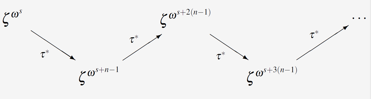
and one can see immediately that $\tau^*$ exchanges the two periods generated by the splitting process. Writing $p_{n,m}$ for the upper period in the diagram and $p_{n,m+2^{n-1}}$ for the lower period, we have for the product:

$$ \begin{align*} \tau^*(p_{n,m}\cdot p_{n,m+2^{n-1}}) &= \tau^*(p_{n,m})\cdot\tau^*( p_{n,m+2^{n-1}}) \\ &= p_{n,m+2^{n-1}} \cdot p_{n,m} \\ &= p_{n,m}\cdot p_{n,m+2^{n-1}} \eqndot \end{align*} $$

Hence, the product of the two daughter-periods of level $n$ is an element of ${\langle \tau^* \rangle}^\dagger,$ that is the fixed field of the automorphism $\tau^{2^{n-1}}.$ This fixed field is generated by adjunction of the periods of level $n-1,$ thus the product is representable as a rational expression of periods of level $n-1.$

This is sufficient to find the quadratic equation, which has the two periods as its zeroes. To show that the rational expression is in fact a linear combination, needs a bit more work.

Final Remark

Here we will stop our excursion into the realm of Galois theory. We have found our Gaussian periods: they dwell in the fixed fields between $\mathbb{Q}$ and $\mathbb{Q}(\zeta),$ which result from the derived series of the Galois group of this field extension. We even found an easy way to show that the product of two periods, generated by splitting, is a rational expression of periods of a lower level.

Let's remark that Gaussian periods are a special case of Gaussian sums. So you may search for the latter, if you want to learn more about the relationship of all the roots among each other according to arithmetic criteria, to quote Gauss once again.